The Honest Number Was 83%
A consumer files a complaint about a financial company. Someone has to decide which product team it belongs to — credit reporting, debt collection, mortgage, checking account — and route it there. Get it wrong and the complaint sits in the wrong queue while a regulatory clock runs.
This paper builds that router. It reads the consumer's free-text narrative and predicts the product category, using 3,831 complaints from the CFPB Consumer Complaint Database.
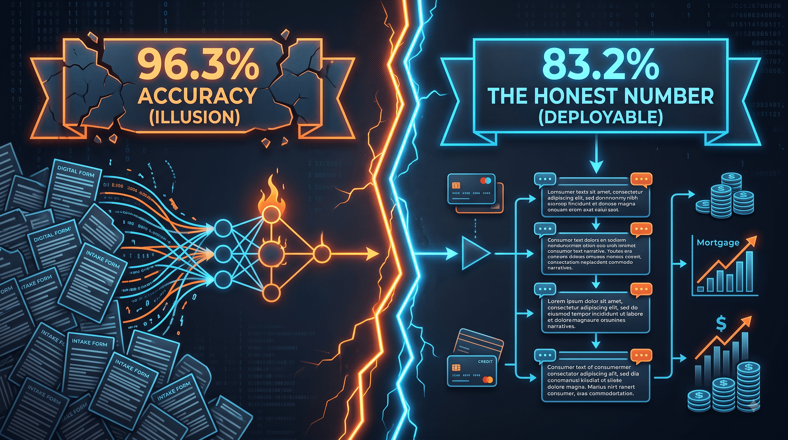
The interesting part is not the model. It is that the same model, trained on the same rows with the same code, reports 96.3% accuracy or 83.2% accuracy depending entirely on whether three innocuous-looking metadata columns are left in the training data. Both numbers are real. Only one of them survives contact with production, and it is the low one.
Why Routing Accuracy Has a Deadline Attached
The CFPB forwards consumer complaints to the company they name. The company is expected to respond within 15 calendar days, with up to 60 calendar days for a final response where the initial one is not final. Complaints are published in the public database once the company responds or after 15 calendar days, whichever comes first.
That is the constraint that makes triage a real problem rather than a classification exercise. A misrouted complaint is not merely an inconvenience — it consumes days of a fixed budget before anyone qualified has read it, and the clock does not pause while it sits in the wrong queue.
The dataset carries its own evidence that this is tracked closely: the Timely response? column reads Yes for 99.2% of rows. Firms are already measured on this. A routing system that quietly degrades that number is not a productivity tool, it is a compliance liability — which is why the deployment question in this paper is not "how accurate is the model" but "under what conditions is it allowed to act without a human."
The Failure That Set the Method
This study replaced an earlier one. That study built a fake-news detector, reached roughly 99% accuracy, and was rejected — because the model had learned that Reuters articles carry a (Reuters) dateline and fake articles do not. It was detecting a publisher's formatting convention, not truth.
Two details from that failure shaped everything here. First, the leak was invisible in every aggregate statistic and obvious the instant anyone printed raw text — it was found by reading, not by describing. Second, a routine preprocessing step (standard stopword removal) had accidentally neutralised a related artifact, which meant the pipeline's apparent robustness was luck.
So this notebook is deliberately structured against that failure mode:
The leakage audit runs first, before a single model is trained.
The metadata columns that would leak are kept in the file on purpose, so that dropping them has to be an explicit, recorded decision rather than an accident of which columns someone happened to select.
Raw text is printed verbatim —
repr(), no paraphrase — because that is what caught the last one.
The finding that generalises past this dataset is in the third section below, and it is not about credit complaints.
Stage 0 — Getting the Data at All
The CFPB Consumer Complaint Database is public. It is also behind a WAF that returns 403 to every scripted request — the API, the bulk archives, any header set, ranged requests included. Only a real browser gets through. There is no scripted path to this data.
The browser download then truncated at 921.6 MB: a valid PK\x03\x04 header with no End-of-Central-Directory record, so no zip tool would open it. Rather than restart a multi-gigabyte download, recover_partial.py raw-inflates the partial deflate stream directly, recovering 3.21 GB of valid CSV — 7,198,079 rows — before the stream hits an invalid block.
The check that makes the salvage usable is the only interesting step here. A truncated file is worthless if the lost tail is a coherent chunk — if the rows were date-sorted, the recovered file would be missing a specific time period and every downstream distribution would be quietly wrong. The rows were verified to be not date-sorted, which makes the loss a random slice rather than a time hole. Without that verification nothing else in this paper would be defensible.
What Is Actually in the File
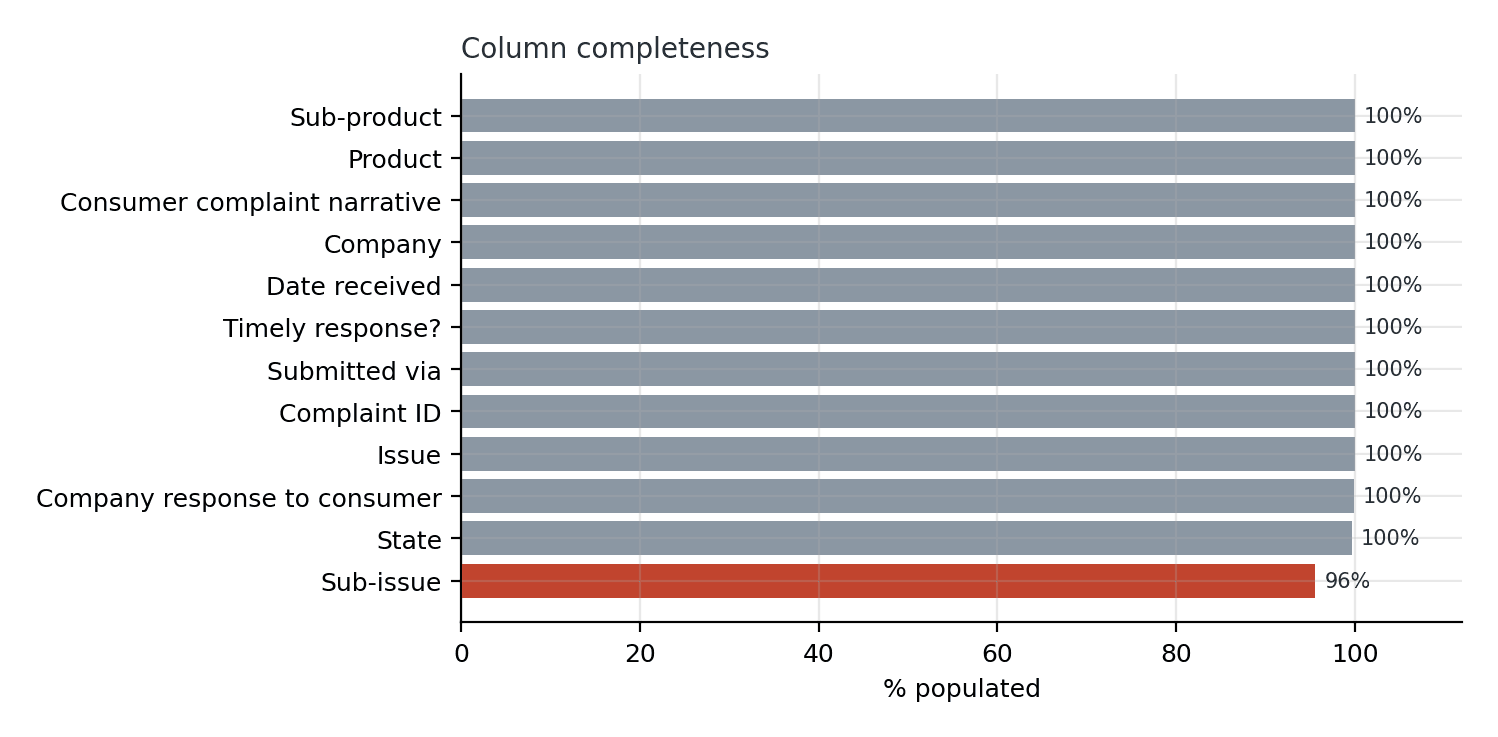
Twelve columns, 3,831 rows. Completeness is high across the board — Sub-issue is the only column with meaningful absence at 4.41% null.
One number on that chart is misleading by construction and worth stating plainly: Consumer complaint narrative is 100% populated only because the file was filtered to narrative-bearing rows. In the raw CFPB database the narrative is optional and present in a minority of complaints. That filter is the single biggest sample-selection decision in the project, and it is not neutral — consumers who take the time to write a narrative are not a random subset of consumers who complain. Every result here is conditional on a complaint having text at all.
The Class Distribution, and Why Accuracy Is the Wrong Metric
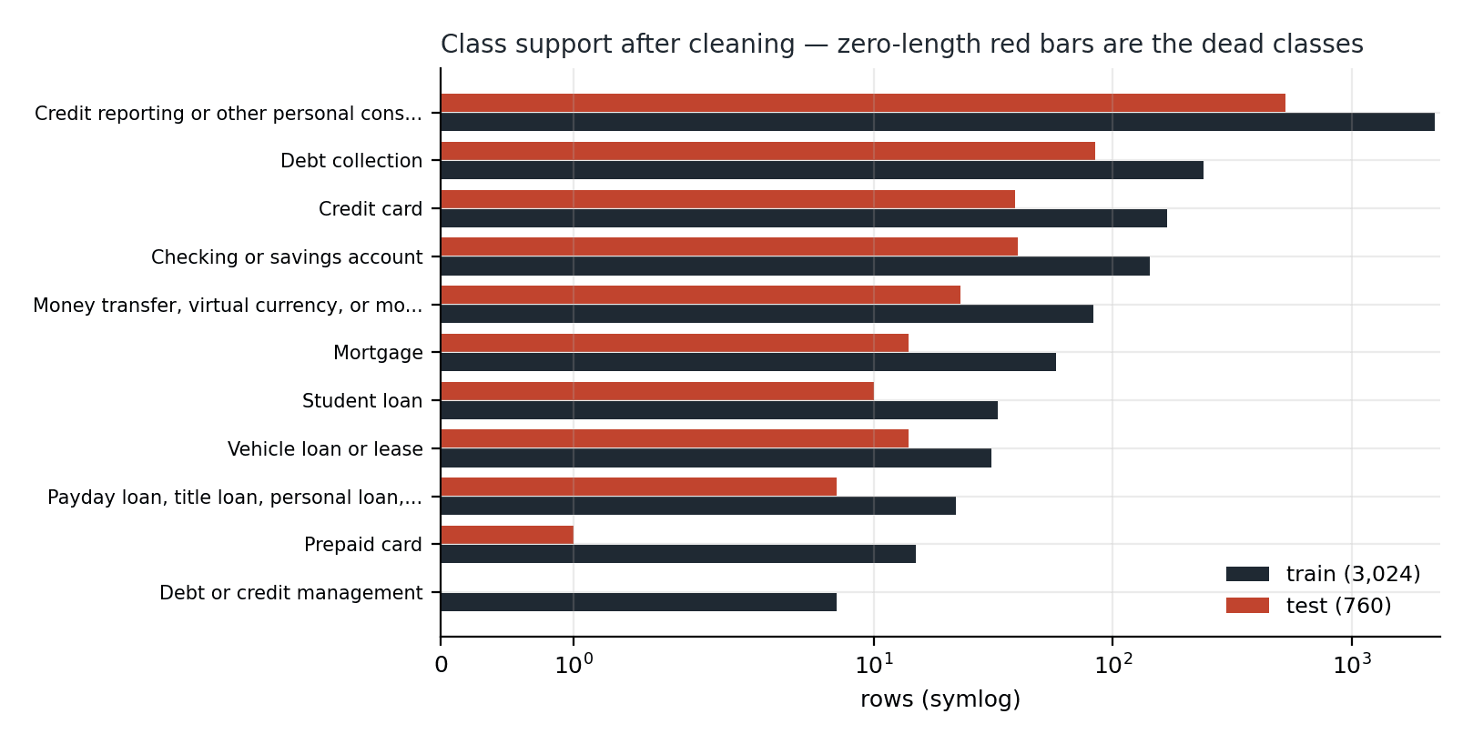
Fifteen distinct Product values, and the distribution is severe:
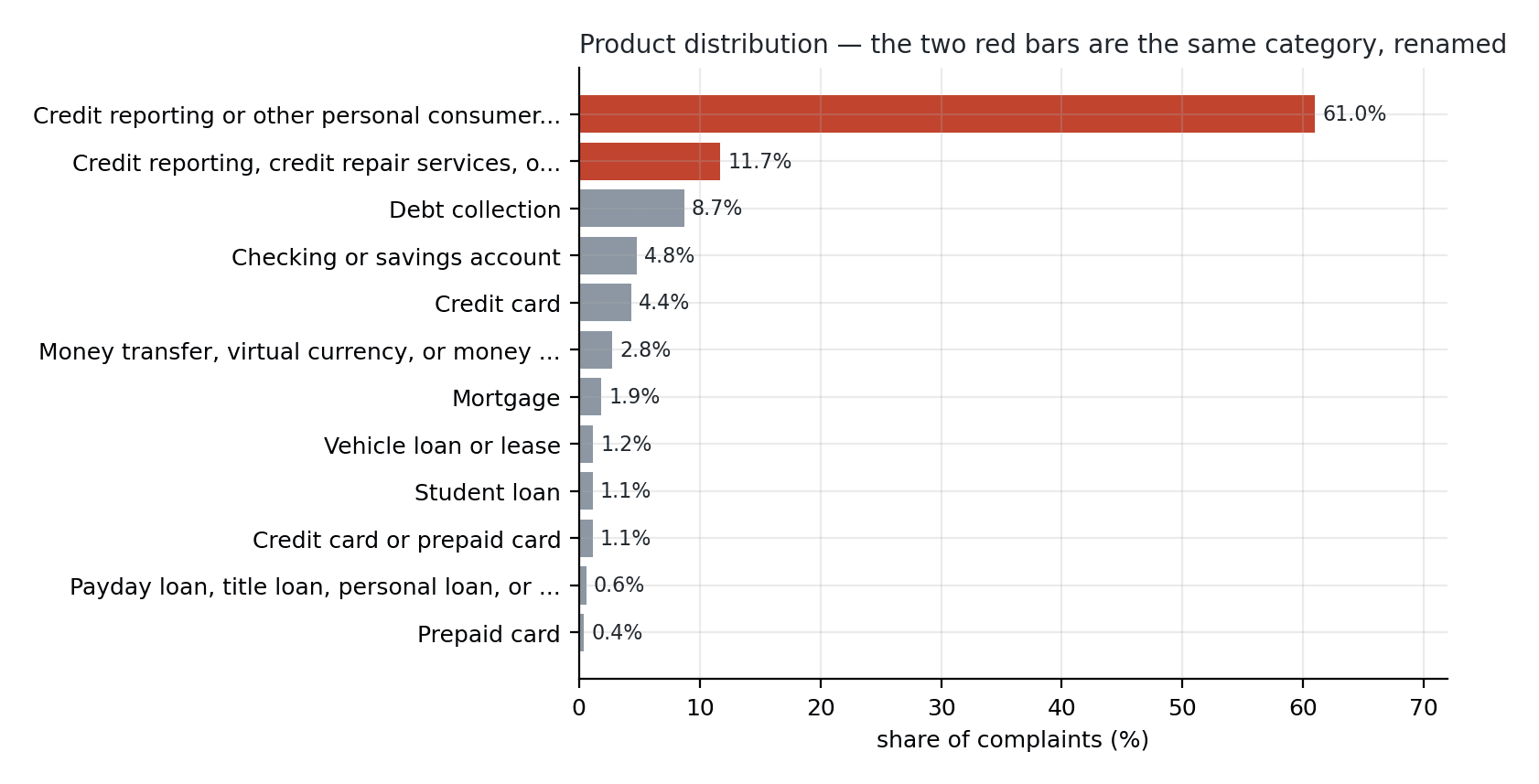
Credit reporting or other personal consumer reports — 2,336 rows (60.98%)
Credit reporting, credit repair services, or other personal consumer reports — 449 (11.72%)
Debt collection — 334 (8.72%)
Checking or savings account — 183 (4.78%)
Credit card — 167 (4.36%)
…then a long tail down to Prepaid card (16), Debt or credit management (7), and a single corrupted row
The imbalance ratio between the largest and smallest class is 2,336 : 1.
The top two entries are the same category under two names — the CFPB renamed it mid-period. Together they are 72.7% of the file. A model that predicts "credit reporting" unconditionally and never reads a word scores 60.98% accuracy, and after the rename is reconciled, closer to 73%.
Macro-F1 is therefore the metric from here on. Accuracy rewards serving the majority; the business cost of failing a tail class is not proportional to its frequency. A mortgage complaint routed to the credit-reporting team is just as late as a credit-reporting complaint would have been, and there are far fewer people watching for it.
The Leakage Audit — The Headline Result
Issue, Sub-issue and Sub-product sit in this file as ordinary-looking columns. They are not ordinary.
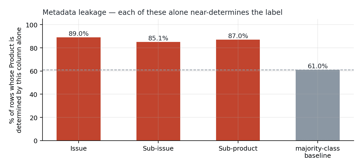
A CFPB intake agent picks Product and Issue from linked dropdowns, in the same sitting. The metadata is not evidence about the complaint — it is a by-product of the labelling act itself. The measure below asks: if you knew only this column's value and always guessed its most common Product, how often would you be right?
Issue— 89.01% (64 distinct values)Sub-product— 87.03% (48 distinct values)Sub-issue— 85.09% (143 distinct values)(majority-class baseline for comparison — 60.98%)
Each of these columns, alone, near-determines the label. All three were excluded as features. Keeping any one of them produces a headline accuracy that measures the intake form, not the complaint text — and critically, at deployment the narrative arrives before anyone has assigned an Issue. Those columns do not exist yet at the moment the routing decision has to be made. Whatever they buy in training is unavailable in production by definition.
This is the same structural failure as the fake-news subject column, in a completely unrelated domain. That is the finding worth carrying to your own work: in any human-curated dataset, the metadata was created by the same person, at the same moment, as the label. It is not independent evidence. Assume leakage until proven otherwise, and prove it with the ablation in section 3.1 rather than with an argument.
Three Text Artifacts, Each With a Modelling Consequence
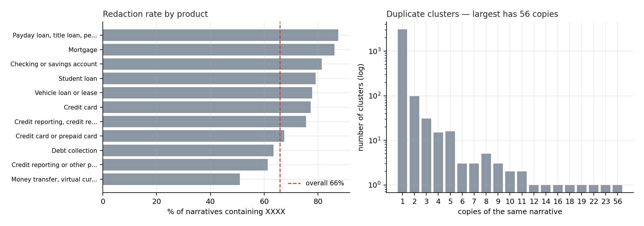
XXXX redaction masks — 65.78% of narratives (2,520 rows). The CFPB scrubs PII before publication, leaving literal XXXX runs. They are frequent enough to be part of the text distribution rather than noise, and xxxx xxxx shows up as a top-weighted feature for the majority class. This is a train/serve skew: a deployed model reads unredacted text it has never seen.
Duplicate narratives — 14.90% (571 rows). Credit-repair services file templated complaints en masse. The largest cluster is 56 identical complaints; 186 clusters contain more than one copy; 3,260 of 3,831 rows are unique. A plain train_test_split would place copies of the same text on both sides of the split for 571 rows — memorisation scored as generalisation. These must be deduped before splitting.
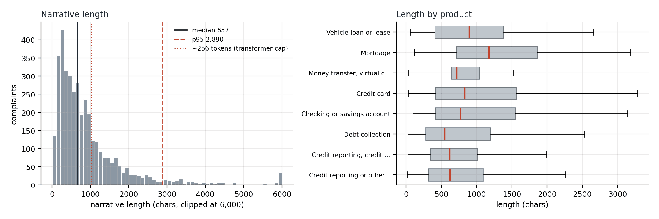
Length — median 657 characters, mean 981, p95 2,890, max 30,592. The p95 narrative runs past 700 tokens, well beyond what a 256-token transformer can read. That single fact carries the caveat on the entire stage-4 comparison.
One check worth doing that came back clean: redaction rate does not vary sharply by class. If XXXX density had correlated with the label, redaction volume would itself have been a leak. It ranges from about 51% to 88% across products with no relationship to the routing target — a negative result, and negative results are the ones nobody publishes.
Taxonomy Drift, and a Date Bug That Hid 18 Months
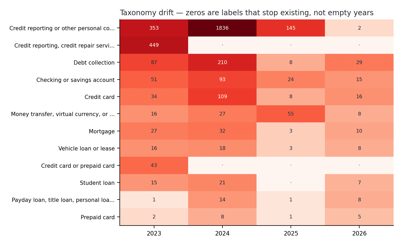
The Product vocabulary is not stable across the period. It carries 14 distinct labels in 2023 and 10 by 2026, and four labels disappear entirely — including the legacy credit-reporting name and Credit card or prepaid card. The same complaint filed two years apart carries two different labels. Any model trained across the whole window is learning a moving target unless the labels are reconciled first.
Alongside it, a smaller bug with a larger blast radius. The Date received column mixes two formats: 2023-07-16 for 3,721 rows and 2026-05-26T07:22:18.000Z for 110. Pandas infers a single format from the leading rows and returns NaT for the rest — so the naive parse reports a maximum date of 2025-01-17 when the true maximum is 2026-07-02.
The failure is quiet and it is directional. Nothing crashes. 110 rows out of 3,831 fail to parse — an easy number to note and move past — and the summary that comes out the other side understates the dataset's coverage by 18 months. A reader planning a temporal split, or checking whether the data covers a policy change, would be working from a wrong end date with no indication anything was wrong. The fix is one argument: format="mixed".
The Column That Is Arguably Legitimate
Company, State, Submitted via and Timely response? are not model features here, but one of them is a genuine judgement call rather than an obvious exclusion.
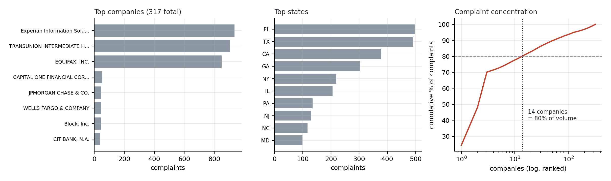
The complaint volume is extraordinarily concentrated: 317 distinct companies, but Experian (24.4%), TransUnion (23.6%) and Equifax (22.2%) are 70.2% of the file between them. Just 14 companies account for 80% of all complaints.
Company is arguably legitimate — a monoline credit bureau really does receive mostly credit-reporting complaints, and that is a true fact about the world, not an artifact. It is also arguably a leak: the model learns the firm's product mix instead of reading the complaint, and with this concentration it could reach a respectable score having learned almost nothing about text.
It is excluded here, on a deployment argument rather than a statistical one. A triage model should generalise to a company it has never seen. A routing system that depends on knowing the recipient is not routing — it is looking up. Worth noting that this is structurally the same trap as the (Reuters) dateline: an identity token inside the input that lets a classifier bypass the actual task.
Submitted via is a different case entirely — it has exactly one distinct value (Web, 100%). It carries zero information and would be silently useless rather than harmful.
Stage 2 — Four Preprocessing Decisions, Each of Which Moves the Score
1. Drop the corrupted row. One row carries the label Credit rurepoA report — bit damage from the salvage, not real data. It was left in the file deliberately as a data-quality tripwire.
2. Merge the legacy taxonomy labels. The renamed credit-reporting category stops being two classes competing with each other. This is the single highest-impact decision in the stage — measured independently, consolidating 14 raw classes to 11 moved macro-F1 from 0.461 to 0.581, +26% relative, from the merge alone.
The honest reading of that gain: merging two classes that were being confused with each other removes that confusion partly by construction. This is not "the model improved," it is "the task was corrected." The correction is legitimate — the two labels genuinely are the same CFPB category before and after a rename — but the win is identifying a mis-specified target, not tuning a model.
3. Drop text-identical groups whose labels disagree. Six narrative groups appear verbatim with two different ground truths. These are unlearnable by construction. This is the label-noise finding, and it returns in stage 5 wearing a disguise.
4. Group-split on the normalised narrative. No duplicate can straddle train and test. Verified overlap: zero.
Result: 3,831 rows → 3,784, 15 classes → 11, split 3,024 train / 760 test. One class (Debt or credit management, 7 rows) lands entirely in train and is absent from test — so no claim of any kind is supportable about it, and that is stated rather than buried.
Stage 3 — The Baseline, and the Gap That Matters
Word and bigram TF-IDF (min_df=2, sublinear scaling, 36,841 features) into a logistic regression with class_weight="balanced". Narrative text only.
macro-F1 — 0.540
weighted-F1 — 0.827
plain accuracy — 0.832
The number to look at is not either of those. It is the 0.287 gap between them. That gap is the imbalance, quantified: the model serves the majority class well (credit reporting, F1 0.92 on 528 test rows) and the tail poorly (Vehicle loan or lease, F1 0.19 on 14 rows). Reporting only the weighted figure would describe this model as 83% effective. Reporting only macro would describe it as 54% effective. Both are true and neither is sufficient alone.
3.1 The Ablation — What the Metadata Would Have Bought
Arguing that a column leaks is weak. Training with it and showing the number a less careful pipeline would have published is not.
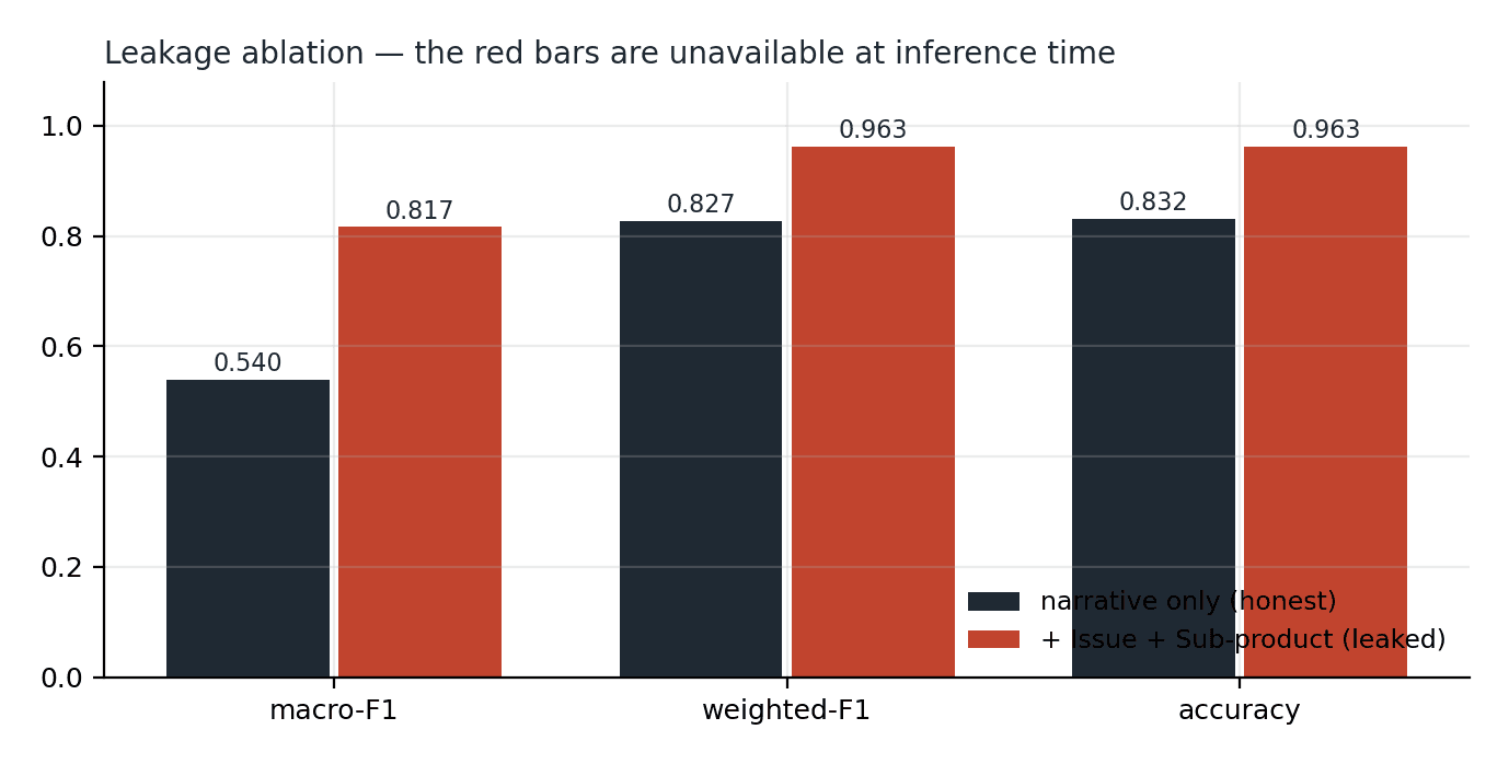
Same model, same split, same code. The only change is appending Issue and Sub-product to the input text:
narrative only (honest) — macro-F1 0.540 · weighted-F1 0.827 · accuracy 0.832
narrative + Issue + Sub-product — macro-F1 0.817 · weighted-F1 0.963 · accuracy 0.963
inflation — +0.277 macro · +0.135 weighted · +0.132 accuracy
A 96.3% complaint router. It would pass review. It would demo well. Macro-F1 jumps by more than half its honest value.
And it is worth nothing at all, because at inference time the narrative arrives before anyone has assigned an Issue — the columns the model depends on do not exist yet. The second row is not a better model. It is the intake form being read back to you.
This is the ablation the fake-news study needed and never got before it was rejected. It costs one extra training run. Publish it next to any headline number that depends on which columns you happened to select.
3.2 What the Model Actually Learned
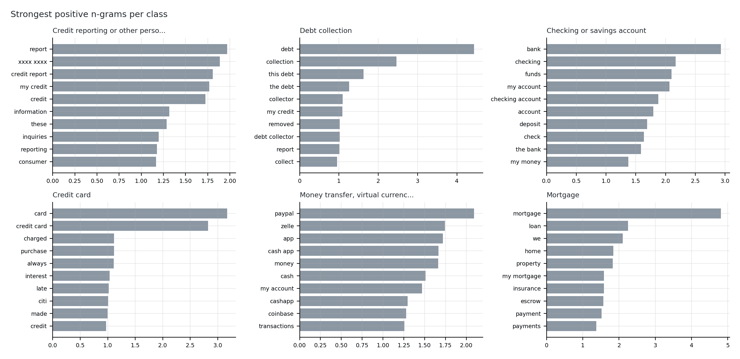
TF-IDF plus logistic regression is fully inspectable — every class has a signed weight per n-gram. This is the interpretability that stage 4 trades away, and in a regulated setting it is not a small thing: a routing decision affecting a legally-timed response may have to be explained to a regulator.
Read the top features as a sanity check. They should look like topic words. If a class's strongest features were formatting artifacts, boilerplate, or company names, that would be another leak.
They pass. debt / collection / collector / validation for debt collection. bank / checking / funds / deposit for checking accounts. paypal / zelle / cash app / coinbase for money transfer. mortgage / escrow / property for mortgage.
Two honest observations against that. The majority class's second-strongest feature is xxxx xxxx — a redaction artifact, not a topic word, and precisely the train/serve skew flagged earlier. And the money-transfer and credit-card classes lean on brand names (paypal, zelle, coinbase, citi). Those are real signal, but they are identity signal: the model has partly learned which brands sit in which product line, which is the same category of shortcut as the Company column that was deliberately excluded — arriving here through the text instead.
Stage 4 — DistilBERT, and Why the Verdict Is Provisional
Same split, same class weighting, so the comparison is like-for-like. CPU-only, so max_length=256, 3 epochs, ~95 minutes.
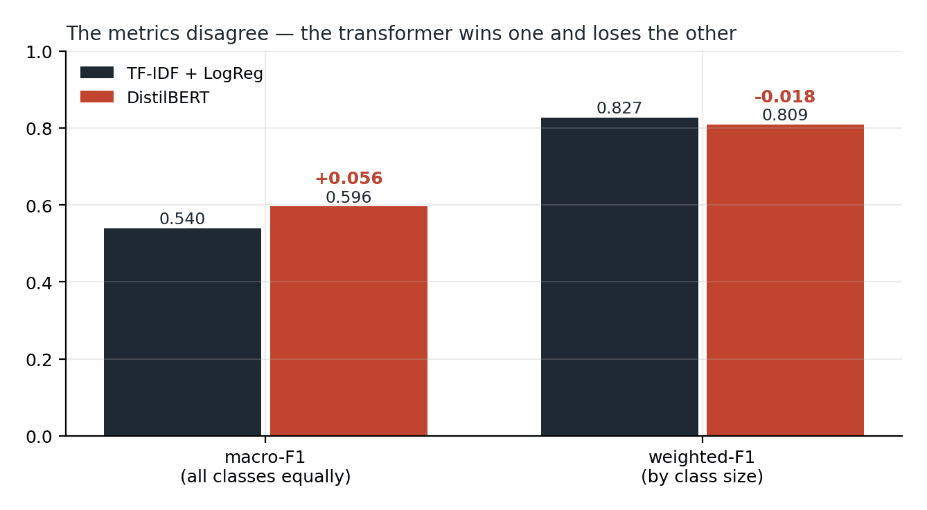
TF-IDF + LogReg — macro 0.540 / weighted 0.827
DistilBERT — macro 0.596 / weighted 0.809
delta — +0.056 macro / −0.018 weighted
The metrics disagree. The transformer wins one and loses the other. It reallocates capacity toward the rare classes and pays for it on the majority. "Which model is better" is therefore not answerable from these numbers — it becomes answerable only once someone decides whether a misrouted prepaid-card complaint costs the same as a misrouted credit-reporting one. The metric choice is the product decision, and it is made before training, not after.
The call is to ship the baseline. A +0.056 macro gain does not justify orders-of-magnitude higher inference cost plus the loss of per-feature interpretability in a regulated setting.
But that conclusion is scale-conditional, and this is its weakest point. Both models saw 3,024 training rows — a limit imposed by an upload constraint in a parallel tool evaluation, not by anything methodological. The real set has 1.32M rows, and transformers scale with data far better than TF-IDF does. The 256-token cap also handicaps DistilBERT specifically, since the p95 narrative exceeds it while TF-IDF reads the full text. At full scale with 512 tokens this comparison could plausibly invert.
The supportable claim is "at 3,024 training rows, the baseline wins." Stating it more broadly would repeat the exact error that got the previous case study rejected.
Stage 5 — Where the Model Fails, Class by Class
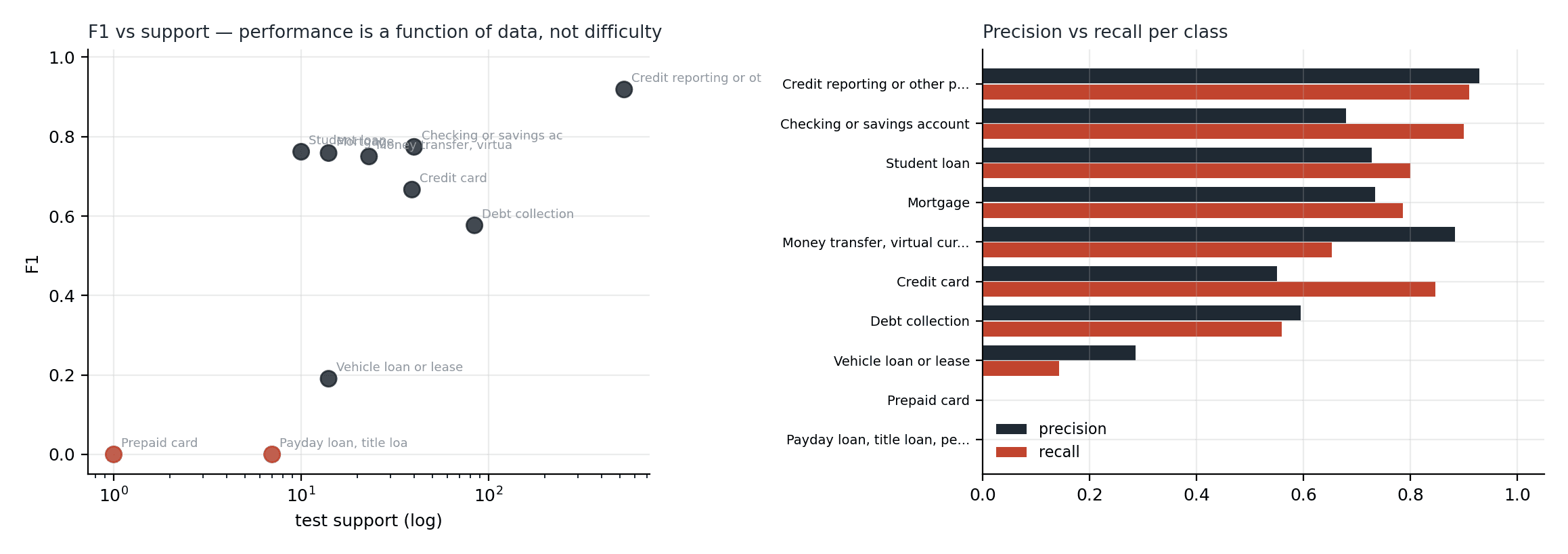
Per-class F1 on the 760-row test set tracks support almost perfectly:
Credit reporting (n=528) — 0.92
Checking or savings account (n=40) — 0.77
Mortgage (n=14) — 0.76 · Student loan (n=10) — 0.76 · Money transfer (n=23) — 0.75
Credit card (n=39) — 0.67
Debt collection (n=84) — 0.58
Vehicle loan or lease (n=14) — 0.19
Payday loan (n=7) — 0.00 · Prepaid card (n=1) — 0.00
Performance is a function of data volume, not task difficulty. Two of the ten classes present in test are unserviceable — the model never predicts them correctly, at all.
Reporting the zeros is not enough. The deployment consequence is that complaints in those categories must be routed by rule or by hand, never by the model, and that has to be written into the routing policy up front rather than discovered in production when a payday-loan complaint quietly lands in the credit-reporting queue.
Debt collection at 0.58 is the interesting failure. It has 84 test rows — not a starvation case — and it still fails. The next section explains why, and the explanation is not "train longer."
Where the Errors Concentrate
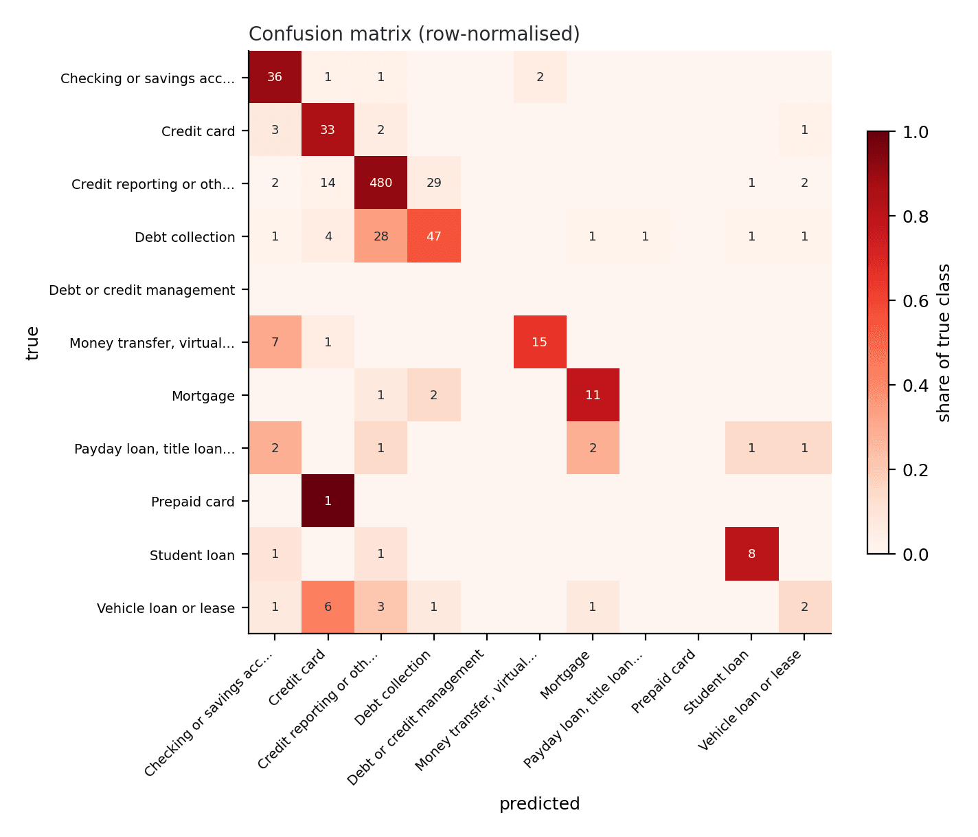
There are 128 errors across 760 test predictions. They are not spread evenly:
29 — Credit reporting → Debt collection (5.5% of that true class)
28 — Debt collection → Credit reporting (33.3% of that true class)
14 — Credit reporting → Credit card (2.7%)
7 — Money transfer → Checking or savings (30.4%)
6 — Vehicle loan or lease → Credit card (42.9%)
The top two pairs are 57 of 128 errors — 45% — and they are the same two classes confused in both directions.
Bidirectional confusion is a specific signature, and it does not mean the model is weak. It means the categories overlap. A consumer disputing a debt that appears on their credit report has genuinely written a complaint that belongs to two products at once, and the CFPB taxonomy forces the intake agent to pick one. A third of all real debt-collection complaints get pulled into credit reporting, which is where the 0.58 F1 comes from.
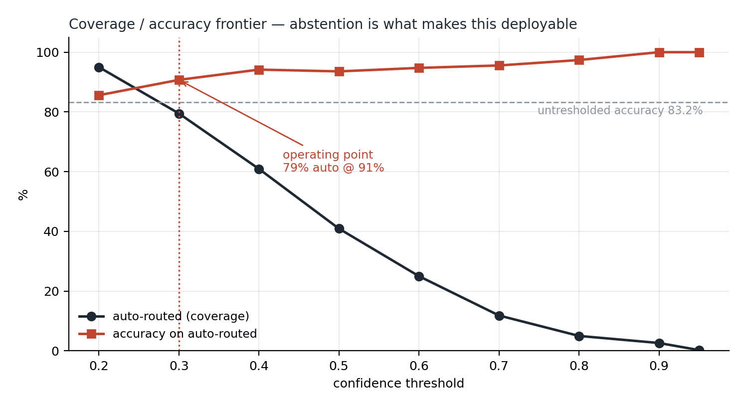
A model at 83% accuracy is one nobody deploys. The same model, permitted to say "I don't know", is deployable — because the question stops being "is the model good enough" and becomes "how many reviewers do we staff."
The Confidence Frontier — The Part That Makes This Shippable
Every number so far describes a model forced to answer every question. Remove that constraint. Route automatically only when the top predicted probability clears a threshold; send everything below it to a human queue.
At a threshold of 0.30: 79.5% of complaints auto-route at 90.7% accuracy, and 20.5% go to human review.
Compare that to the unthresholded model — 83.2% accuracy at 100% coverage — and the trade is clear. Giving up a fifth of the volume buys +7.5 points of accuracy on everything that remains automated. The model did not change. Not one weight was retrained. The only difference is that it is allowed to abstain.
This reframes the deployment conversation entirely. "Is 83% good enough to route complaints?" has no good answer. "Do we have capacity to review 1 in 5 complaints, in exchange for automating the other 4 at 91%?" is a staffing question with a number attached, and an operations manager can answer it.
The threshold is also the control surface. Tighten it to 0.40 and accuracy goes to 94.2% with 60.9% coverage. Anyone can move that dial as capacity changes without retraining anything.
Is the Confidence Trustworthy?
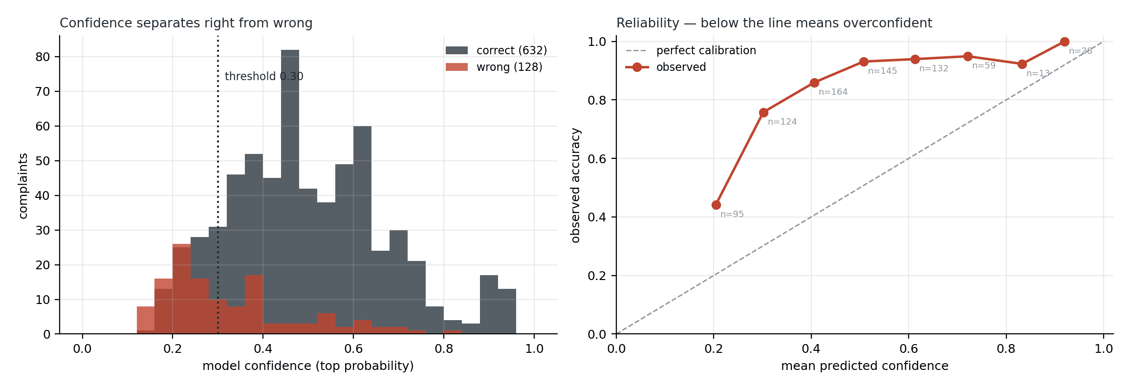
Thresholding only works if the probability means something, so two checks — and both turned up something worth reporting rather than the clean result that was expected.
The frontier is not perfectly monotone. Accuracy on auto-routed complaints goes 94.2% at threshold 0.40 and 93.6% at 0.50 — it dips where it should only rise. The dip is small and lands where the sample gets thin, so the most likely explanation is noise rather than broken probabilities. But the plan going in was to treat monotonicity as a pass/fail safety check, and the honest report is that it did not strictly pass. Stating "the frontier is monotone" would have been the easy sentence and it would have been false.
The model is under-confident, not overconfident. The reliability curve sits consistently above the diagonal: in the band where it reports about 0.30 confidence it is right 76% of the time; at 0.51 it is right 93%. Its stated probabilities systematically understate its accuracy.
That is the benign direction to be wrong in — overconfidence is what pushes a wrong answer past the threshold into auto-routing — but it has a concrete consequence that is easy to misread. The 0.30 operating point is not a "low-confidence" setting. It looks alarmingly permissive and is not, because 0.30 from this model means roughly 76% and above. With 11 classes and balanced class weights, the softmax is simply compressed. Anyone tuning this threshold by intuition, or transferring 0.30 to a differently-shaped model, would get badly burned. The raw probabilities are not calibrated, and the threshold is only meaningful against this frontier.
The Dangerous Errors — Confidently Wrong
Low-confidence errors are harmless; the queue catches them. The errors that matter are the ones the model was sure about, because those clear the threshold and get auto-routed. So read them raw.
All five of the highest-confidence errors are the same thing: a consumer disputing a debt that appears on their credit report.
This is the stage-1 label-noise finding coming back wearing a different hat. These are exactly the narratives that appeared verbatim in stage 2 carrying two different ground-truth labels — the six conflicting groups that were dropped as unlearnable. The model is not wrong about these. The taxonomy is ambiguous and the ground truth contradicts itself.
Two consequences that matter more than the F1 number:
Part of the residual error is irreducible. No architecture removes error that comes from contradictory labels. Knowing this is what tells you when to stop modelling, and it is the single finding that saves the most time — it is the difference between shipping and spending another month chasing a ceiling that does not exist.
The fix is not a better classifier. It is merging the two categories, moving to multi-label, or writing this slice into the human queue by policy. That is a taxonomy decision and an ops decision. No amount of model work reaches it.
Problems We Hit, Including Our Own
A clean write-up hides the process. Here is what actually went wrong.
The transformer run died and could not be recovered in the assistant's environment. The AI analysis tool used for the parallel evaluation track executes Python and produced genuine artifacts for every earlier stage — but importing transformers destabilised its execution kernel permanently, after which even a bare print() failed. Stage 4 had to move to a local run. The lesson generalises: confirming that a sandbox executes pandas and scikit-learn tells you nothing about whether it can load a deep-learning stack. Those are very different footprints, and the assumption that stage 3 working implied stage 4 would work was recorded, then had to be corrected.
What the tool did next is the most valuable result in the evaluation. With no valid predictions, it stated explicitly that no transformer macro-F1, weighted-F1, per-class recall or confusion matrix should be treated as available, and produced a run-status document instead of numbers. A fabricated macro-F1 of "0.62" would have looked entirely reasonable, would have matched expectations, and would have been nearly impossible to catch without independent reproduction. It under-investigates; it does not invent. Those are very different risk profiles, and the second is far more dangerous.
A disclosed caveat that turned out to have a measurable cost. The tool flagged, unprompted, that its logistic regression hit max_iter. That reads like boilerplate. It was not: its macro-F1 came in at 0.4357 against 0.540 from the independent rebuild, while weighted-F1 agreed closely (0.819 vs 0.827). An under-converged solver degrades rare classes most, and rare classes are exactly what macro-F1 measures. The caveat was honest, it was ignored, and it cost 0.10 macro-F1 — visible only because the run was independently reproduced.
Our own failure: the monotonicity claim. The stage-5 reference notes recorded "frontier monotone: thr 0.20→0.95 gives acc 85.6%→100%." The endpoints are correct and the intermediate values were in the same table, where accuracy visibly dips from 94.2% to 93.6%. Nobody checked the middle. The claim was written from the shape the frontier was expected to have, and the data contradicting it was already on screen. It is corrected in this paper because the alternative — quietly deleting it — is the failure this whole line of work exists to document.
Charts could not be rendered inline. The assistant saves charts as downloadable PNG artifacts rather than displaying them in the conversation, so it cannot show a visual while explaining it. Iterative visual review — "that axis is unreadable, redo it" — is considerably slower than it should be.
Limitations
Trained on 3,024 rows. The full set has 1.32M. The baseline-beats-transformer verdict is conditional on that size and could invert at scale. This is the highest-value open item in the project and it is not a small caveat — it is the one claim most likely to be wrong.
The 256-token cap handicaps DistilBERT specifically. p95 narratives exceed it. TF-IDF reads the full text; the transformer does not. The comparison is like-for-like on data and unfair on architecture.
760 test rows, 10 of 11 classes present. One class has a single test row. No claim about the tail is statistically supportable, and the two 0.00 F1 scores are as much a statement about test support as about the model.
The sample's duplicate rate is not the population's. The sample reads 14.90%; the full 1.32M-row set is 37.48%, because random sampling breaks duplicate clusters apart. Any figure here must be compared against the sample's own numbers, never the full set's.
XXXX redaction is an unmodelled train/serve skew. Production text arrives unredacted. This model has never seen an unredacted narrative, and xxxx xxxx is one of its strongest majority-class features.
Narrative-bearing complaints are not a random sample of complaints. Everything here is conditional on the consumer having written free text.
The probabilities are not calibrated. The threshold works empirically against this frontier and does not transfer to another model.
What Would Actually Improve This
Re-run stage 4 at full scale with 512 tokens on a GPU and settle the baseline-versus-transformer question properly — it is the only open item that could reverse a stated conclusion. Calibrate the probabilities so the threshold has a meaning that transfers, rather than one that holds only against this particular frontier. Attach an explicit cost matrix: a misrouted mortgage complaint and a misrouted credit-reporting complaint are not the same event, and every model here was trained as though they were. Escalate the Debt collection ↔ Credit reporting overlap to whoever owns the taxonomy, because 45% of the error budget sits in a pair of categories that a human intake agent also cannot cleanly separate. And expose the threshold as an operator-adjustable control rather than a constant buried in the code — the whole point of the frontier is that the right operating point is a staffing decision, and staffing changes.
Conclusion
The model that routes CFPB complaints from narrative text alone scores macro-F1 0.540 and 83.2% accuracy. That number looks like a failure and it is the honest one.
The 96.3% version exists. It is one line of code away — append Issue and Sub-product to the input — and it would survive most reviews, because nothing about it looks wrong. It fails for a reason no metric can surface: those columns are filled in by the same person who assigned the label, in the same sitting, and at the moment a real complaint arrives they are empty. The leak is not statistical. It is temporal, and no amount of cross-validation finds it.
Two things to take away.
On the data: in any human-curated dataset, the metadata was created by the same person, at the same moment, as the label. It is not independent evidence about the thing you are predicting — it is a fingerprint of the labelling act. The fake-news study learned a (Reuters) dateline; this one could have learned an intake dropdown. Different domains, same failure. Assume it, then prove it with an ablation and publish both numbers.
On the deployment: 83.2% is not a verdict, it is an input. The same model that is unshippable when forced to answer everything auto-routes 79.5% of complaints at 90.7% accuracy the moment it is allowed to abstain — no retraining, one threshold. The most valuable thing a model can learn to say is that it does not know, and the most common reason that capability is missing is that nobody asked for it.
29 July 2026
EdgeGuard: AI-Driven Predictive Maintenance for Power Transformers
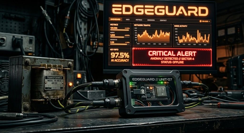
Power transformers are among the most critical assets in electrical distribution infrastructure. Their unexpected failure can result in power outages, safety hazards, equipment damage, expensive repairs, and long service interruptions. Traditional transformer maintenance practices often rely on periodic manual inspection, offline testing, or run-to-failure maintenance. These methods are expensive, slow, labor-intensive, and unable to detect rapidly developing faults in real time. EdgeGuard is an AI-driven, edge-computing predictive maintenance system designed to continuously monitor transformer health and forecast failures before catastrophic damage occurs. The system acts as a retrofittable “Digital Doctor” for distribution transformers by combining low-cost industrial sensors, an ESP32 microcontroller, local intelligence, machine learning-based risk prediction, autonomous relay control, and a real-time web dashboard. The proposed system monitors six major transformer health indicators: temperature, humidity, vibration, oil level, current, and voltage. These signals are normalized and processed through a Multi-Layer Perceptron neural network to classify transformer condition and estimate failure risk. If the predicted risk crosses a critical threshold of 80%, EdgeGuard automatically triggers a relay through GPIO 26 to isolate the transformer from the electrical network. The system also supports secure remote control, dashboard monitoring, API-key-based hardware authentication, JWT-based user access, WebSocket live updates, and automatic live-hardware detection. With an estimated deployment cost of approximately ₹3,850, EdgeGuard offers a low-cost alternative to conventional transformer monitoring systems. Its cloud-independent operation and edge-based decision-making make it especially useful for rural and semi-urban distribution grids where connectivity and maintenance resources are limited.

28 July 2026
ANALYZING TOXIC USER BEHAVIOR AND RISK PATTERNS IN ONLINE GAMING PLATFORMS
This study shows that behavioral data alone can't reliably predict gaming toxicity — but a risk-based model combining behavioral and engineered features does a much better job of flagging the small segment of high-risk users driving disproportionate harm.
28 July 2026
Predicting Smart Grid Stability Using Terno Agentic AI
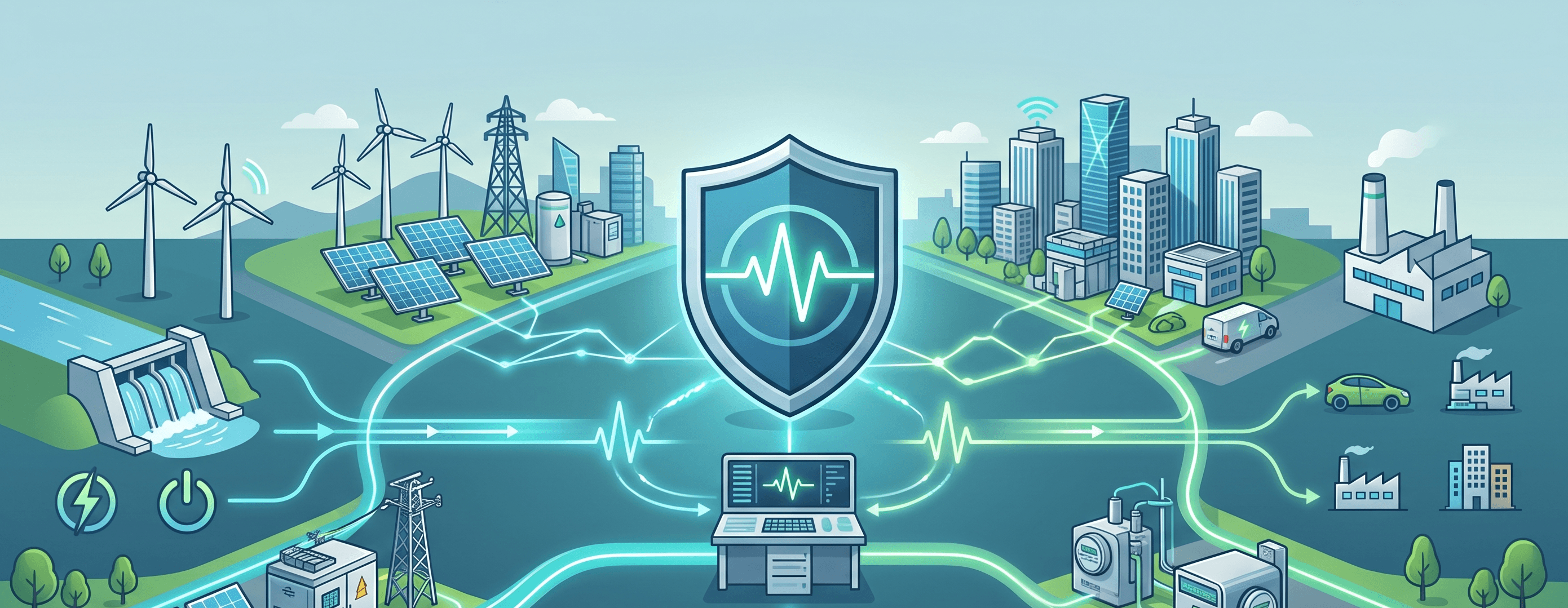
Analyzing 60,000 smart grid records with Terno AI, XGBoost hits 98% accuracy and a 0.998 ROC-AUC in classifying grid stability — with price elasticity and reaction-time features doing the heavy lifting.