
Bitcoin trades around the clock, swinging wildly even within a single 15-minute window. That volatility is exactly why short-term price prediction is so tempting — and so hard. A recent whitepaper takes on the challenge directly: using over seven years of high-frequency trading data, it builds and tests machine learning models designed to predict Bitcoin's closing price just 15 minutes into the future.
The results are a genuinely useful case study in both the promise and the pitfalls of financial time-series modeling — including a cautionary tale about a model that looked great in training and then completely fell apart on real test data.
Here's what the analysis found.
The Problem: Predicting the Unpredictable
Bitcoin's continuous, highly volatile trading creates both an opportunity and a challenge. High-frequency data — like 15-minute OHLCV (Open, High, Low, Close, Volume) intervals — makes it possible to study fine-grained market behavior. But extracting real signal from that much noisy, fast-moving data requires careful, structured analysis.
The objective was specific: predict the next 15-minute closing price of Bitcoin using historical OHLCV data and trading activity features. That means building a regression model, not just describing past trends — a model that traders, analysts, or automated trading systems could actually use to make short-term decisions like intraday trading or scalping.
The key challenges baked into this problem:
High volatility — frequent, unpredictable price swings even in short windows
Large data volume — over 285,000 time-series records to process
Market noise — irregular fluctuations and outliers
Feature relevance — figuring out which variables actually matter
Time dependency — capturing the sequential nature of the data correctly
The Dataset
The study used a high-frequency Bitcoin OHLCV dataset covering January 2018 to January 2025, at 15-minute intervals:
285,069 rows × 12 columns initially (285,068 after processing)
Two time columns (Open time, Close time), four price columns (Open, High, Low, Close), and five volume/activity columns (Volume, Quote asset volume, Number of trades, Taker buy base asset volume, Taker buy quote asset volume)
A constant "Ignore" column that carried no analytical value
The scale of price movement in the dataset is a good snapshot of Bitcoin's history: the opening price ranged from $3,166.11 to $126,011.18, with an average of $38,080.76. Trading volume peaked at over 40,371 BTC in a single 15-minute interval, and the number of trades in a single interval hit over 1.75 million.
Preprocessing
Four straightforward steps prepared the raw data for modeling:
- Converted Open time and Close time to proper datetime format
- Created the target variable —
target_close_next_15m— by shifting the Close price back one step, representing the next interval's closing price - Removed the final row, which had no target value after the shift
- Left all original feature values unfiltered and untransformed, to keep the modeling process free of preprocessing bias
Exploratory Data Analysis: What the Data Actually Looks Like
A Clean Dataset, Which Is Rare for Financial Data
A full data quality check found: no missing values, no duplicate rows, and one constant column (Ignore) that was removed. The final clean shape was 285,068 rows × 12 columns — a genuinely tidy starting point, which isn't always a given with real-world financial datasets.
Price and Volume Statistics
| Feature | Mean | Std Dev | Min | Max |
|---|---|---|---|---|
| Open | 38,080.65 | 32,507.50 | 3,166.11 | 126,011.18 |
| High | 38,155.02 | 32,554.90 | 3,174.78 | 126,199.63 |
| Low | 38,003.79 | 32,458.91 | 3,156.26 | 125,648.01 |
| Close | 38,080.84 | 32,507.51 | 3,167.07 | 126,011.18 |
| Volume | 672.71 | 1,075.77 | 0.00 | 40,371.41 |
| Target (Next Close) | 38,081.03 | 32,507.53 | 3,167.07 | 126,011.18 |
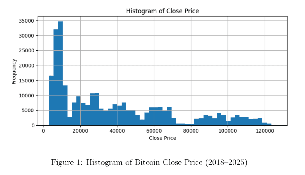
The close price distribution clearly reflects Bitcoin's multi-phase history — distinct clusters at different price levels correspond to different bull and bear market eras rather than one smooth distribution.
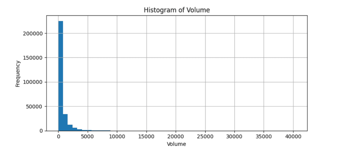
Volume, by contrast, is heavily right-skewed: most 15-minute intervals see relatively low trading volume, punctuated by occasional extreme spikes during high-activity periods. The wide swings in both price and volume are consistent with Bitcoin's well-known volatility — outliers here aren't data errors, they're the market behaving exactly as expected.
Time Coverage Is Solid
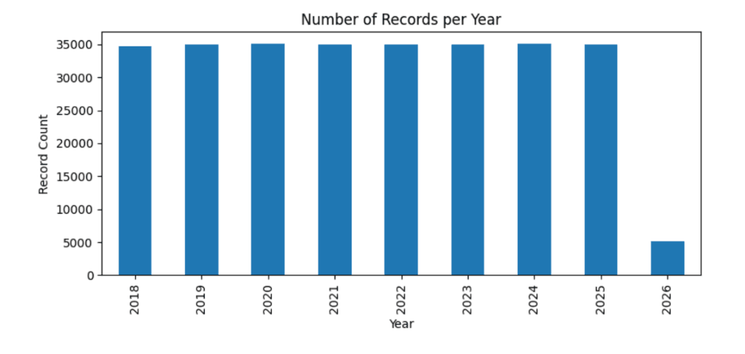
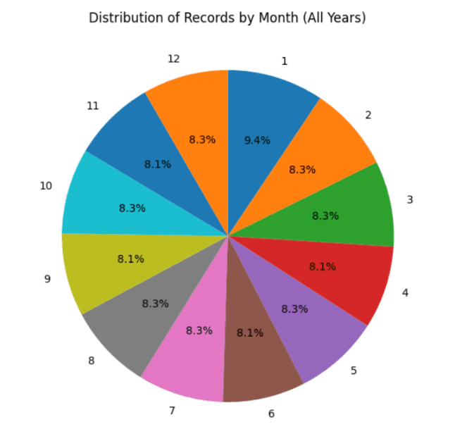
Each complete year from 2018–2025 contributed roughly 35,000 records, with monthly distribution nearly uniform (8.1–9.4% of records per month) and no missing months or irregular gaps. That consistency matters — a time-series model is only as good as the continuity of the sequence it's trained on.
The Strongest Predictor Is Hiding in Plain Sight
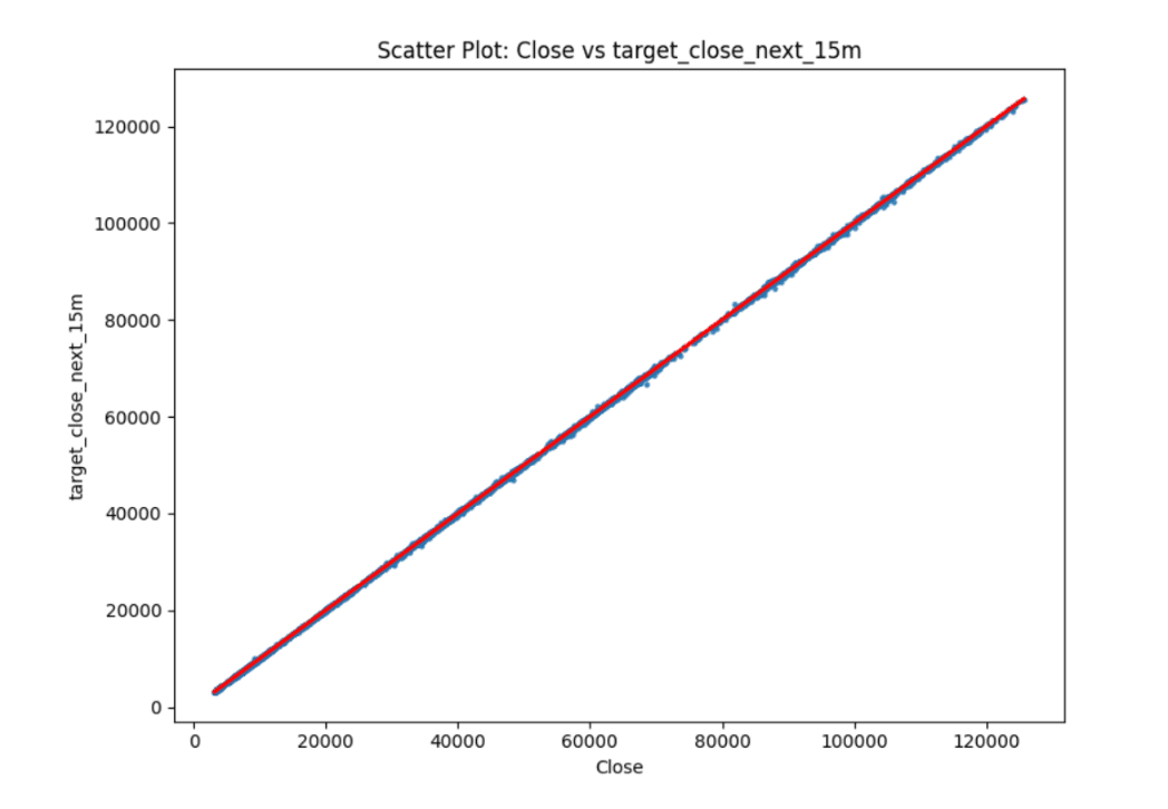
The relationship between the current close price and the next interval's close price is about as close to a straight line as real-world data gets — a correlation of 0.9999. High, Low, and Open all show similarly strong correlations with the target, simply because prices don't teleport between adjacent 15-minute windows.
Number of Trades shows a moderate correlation (0.3308), while volume-related features are weak predictors on their own (roughly ±0.18). In short: the current close price is overwhelmingly the strongest single predictor, while volume and trade activity contribute comparatively little direct signal.
Too Much of a Good Thing: Multicollinearity
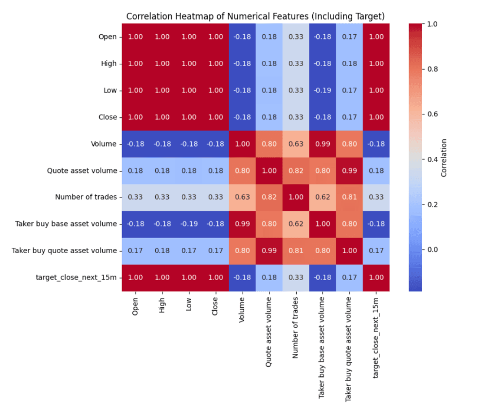
The flip side of that strong correlation is a multicollinearity problem. Open, High, Low, and Close are all nearly perfectly correlated with each other (≈1.0), with a Variance Inflation Factor over 600,000 — an extreme level of redundancy. Volume-related features also correlate strongly with each other (up to 0.99), with VIF over 150. Only Number of Trades showed low multicollinearity (VIF ≈ 5.18).
Why this matters: Feeding a regression model a set of near-duplicate features destabilizes it, inflates variance, and makes the results harder to interpret — so this had to be addressed before modeling.
Trimming Down to What Actually Matters
Based on the multicollinearity analysis, feature selection kept only: Close, Volume, Quote asset volume, and Number of trades — dropping Open, High, and Low (redundant with Close), the Taker buy volume columns (highly correlated with existing volume features), and the constant Ignore column.
Engineering Features That Capture Time
To give the model a better sense of momentum and recent volatility, the study engineered:
Lag features:
close_lag_1,close_lag_2,close_lag_3Rolling statistics:
rolling_mean_3,rolling_std_3A volume lag:
volume_lag_1
After this step, the dataset contained 285,065 rows with 10 input features and 1 target — lag features to capture short-term momentum, rolling features to capture local trend and volatility.
Splitting the Data the Right Way
Rather than randomly shuffling the data (which would leak future information into training), a time-aware 80/20 split preserved chronological order:
Training: 2018 to July 2024 (228,052 rows)
Testing: July 2024 to February 2026 (57,013 rows)
This matters enormously for financial time-series modeling — a model that's accidentally trained on "future" data will look artificially good and fail in real deployment.
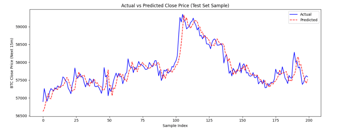
Building the Models: Three Approaches, One Clear Winner
Three regression models were trained and evaluated using RMSE, MAE, and R².
Linear Regression: A Strong, Stable Baseline
Train: RMSE 302.24, MAE 74.32, R² 0.99974
Test: RMSE 295.63, MAE 190.65, R² 0.99975
The close alignment between training and test metrics shows strong generalization with no overfitting — largely thanks to the strong autocorrelation in the price series and the predictive power of the lag features.
Random Forest: Comparable Performance, Mild Overfitting
Train: RMSE 74.13, MAE 19.13
Test: RMSE 295.41, MAE 190.41, R² 0.99975
Performance on the test set was essentially on par with Linear Regression, though the sizeable gap between training and test error signals some mild overfitting. Feature importance analysis confirmed that Close and its lagged versions were the dominant predictors, with rolling statistics contributing secondarily and volume/trade features adding only marginal value.
XGBoost: A Cautionary Tale in Overfitting
Train: RMSE 140.80, MAE 83.43, R² 0.99994
Test: RMSE 26,489.13, MAE 21,501.34, R² −1.046
This is the standout finding of the whole study: XGBoost looked excellent during training — arguably the best of the three models — and then completely collapsed on the test set, performing worse than simply predicting the average price every time (a negative R² means exactly that). Feature importance revealed the problem: nearly 80% of the model's decision-making was concentrated in a single feature, close_lag_2, with everything else contributing almost nothing. That's a textbook sign of severe overfitting in its default configuration — a strong reminder that strong training metrics alone say nothing about real-world reliability.
Model Comparison
| Model | Split | RMSE | MAE | R² | Status |
|---|---|---|---|---|---|
| Linear Regression | Train | 302.24 | 74.32 | 0.99974 | Stable |
| Test | 295.63 | 190.65 | 0.99975 | Stable | |
| Random Forest | Train | 74.13 | 19.13 | 0.99998 | Good |
| Test | 295.41 | 190.41 | 0.99975 | Good | |
| XGBoost | Train | 140.80 | 83.43 | 0.99994 | Good |
| Test | 26,489.13 | 21,501.34 | −1.046 | Overfit | |
| Random Forest (Tuned) | Train | — | — | 0.99982 | Best |
| Test | 260.12 | 170.56 | 0.99980 | Best |
Tuning the Winner
To address Random Forest's mild overfitting, hyperparameter tuning via randomized search with cross-validation found an optimal configuration: n_estimators=200, max_depth=10, min_samples_split=5, min_samples_leaf=2. Post-tuning results:
Test RMSE: dropped from 295.28 to 260.12
Test MAE: dropped from 190.12 to 170.56
Test R²: improved to 0.99980
The narrowing gap between training and test error confirms a healthier bias-variance balance and stronger generalization — making the tuned Random Forest the top-performing model overall, combining the lowest test RMSE, the highest R², and the best balance between fitting the data and generalizing to new data.
Final Insights
A few clear patterns ran through the entire analysis:
Strong autocorrelation drives predictability. Recent closing prices — and their lagged versions — are by far the most powerful predictors of the next price point.
Feature engineering pays off. Lag and rolling statistics meaningfully improved the models' ability to capture short-term momentum and volatility beyond what raw OHLCV data alone could offer.
Price dominates; volume and trades are secondary. Across every model, price-based features consistently outweighed volume and trade activity in predictive importance.
Data quality was excellent from the start — minimal missing values, no meaningful anomalies, and consistent time coverage across the full 2018–2025 span.
Model choice matters more than raw training performance. XGBoost's collapse on the test set is the clearest possible illustration that a model's training-set numbers can be actively misleading if the model hasn't generalized.
Business and Practical Implications
The tuned Random Forest model shows real potential for applications like algorithmic trading, portfolio optimization, and risk management — particularly for generating short-term trading signals under normal market conditions. But it comes with an important limitation: the model relies entirely on historical price and volume data. It doesn't factor in market sentiment, macroeconomic indicators, or breaking news — all of which can move cryptocurrency prices sharply and suddenly. For any serious financial decision-making, this kind of model should be one input among several, not a stand-alone signal.
Key Takeaways
- The current close price is the single strongest predictor of the next 15-minute price — correlation of 0.9999 — but that same strength creates severe multicollinearity that has to be addressed before modeling.
- Lag and rolling features substantially improve prediction quality by capturing short-term momentum and local volatility that raw price data alone misses.
- A time-aware train-test split is non-negotiable for financial time series — shuffling the data would leak future information and produce falsely optimistic results.
- Training performance can be dangerously misleading. XGBoost's near-perfect training scores masked catastrophic real-world failure — always validate on a proper held-out test set before trusting a model.
- Tuned Random Forest strikes the best balance of accuracy and generalization, making it the most production-ready of the three models tested.
- No model here accounts for the "unknown unknowns" — sentiment, news, and macro shocks remain outside its scope, and should be layered in separately for real trading decisions.
Why This Matters
This case study is a genuinely instructive look at short-term financial forecasting — not because it hands traders a magic prediction engine, but because it walks through the real discipline required to build one responsibly: rigorous multicollinearity checks, careful time-aware splitting, and a healthy skepticism toward models that look "too good" on paper. The gap between XGBoost's training and test performance is worth remembering any time a model's numbers seem almost too clean — because in fast-moving, noisy domains like crypto markets, that's often exactly the warning sign.
Read the full white paper here

18 August 2026
The Honest Number Was 83%: Leakage, Abstention, and a Complaint Router You Can Actually Deploy
The same complaint-routing model scores 96.3% or 83.2% depending on which three columns you leave in the training data. The high number is the intake form being read back to you. This is what the leakage audit found before a single model was trained, why 83.2% is the honest figure, and how the same model — given permission to say "I don't know" — becomes deployable at 90.7% accuracy on 79.5% of traffic.
29 July 2026
EdgeGuard: AI-Driven Predictive Maintenance for Power Transformers
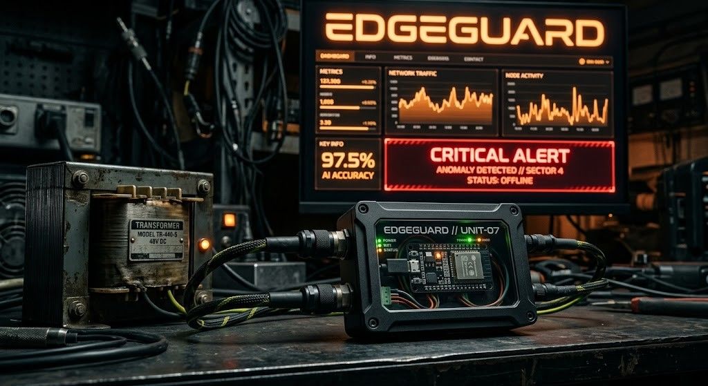
Power transformers are among the most critical assets in electrical distribution infrastructure. Their unexpected failure can result in power outages, safety hazards, equipment damage, expensive repairs, and long service interruptions. Traditional transformer maintenance practices often rely on periodic manual inspection, offline testing, or run-to-failure maintenance. These methods are expensive, slow, labor-intensive, and unable to detect rapidly developing faults in real time. EdgeGuard is an AI-driven, edge-computing predictive maintenance system designed to continuously monitor transformer health and forecast failures before catastrophic damage occurs. The system acts as a retrofittable “Digital Doctor” for distribution transformers by combining low-cost industrial sensors, an ESP32 microcontroller, local intelligence, machine learning-based risk prediction, autonomous relay control, and a real-time web dashboard. The proposed system monitors six major transformer health indicators: temperature, humidity, vibration, oil level, current, and voltage. These signals are normalized and processed through a Multi-Layer Perceptron neural network to classify transformer condition and estimate failure risk. If the predicted risk crosses a critical threshold of 80%, EdgeGuard automatically triggers a relay through GPIO 26 to isolate the transformer from the electrical network. The system also supports secure remote control, dashboard monitoring, API-key-based hardware authentication, JWT-based user access, WebSocket live updates, and automatic live-hardware detection. With an estimated deployment cost of approximately ₹3,850, EdgeGuard offers a low-cost alternative to conventional transformer monitoring systems. Its cloud-independent operation and edge-based decision-making make it especially useful for rural and semi-urban distribution grids where connectivity and maintenance resources are limited.

28 July 2026
ANALYZING TOXIC USER BEHAVIOR AND RISK PATTERNS IN ONLINE GAMING PLATFORMS
This study shows that behavioral data alone can't reliably predict gaming toxicity — but a risk-based model combining behavioral and engineered features does a much better job of flagging the small segment of high-risk users driving disproportionate harm.