
Executive Summary
Accurate delivery time prediction is a key challenge in logistics systems, directly affecting customer satisfaction and operational efficiency. This project focuses on predicting delivery time using historical data from Porter's delivery operations, where multiple factors such as order details, store attributes, and real-time delivery conditions influence outcomes. Traditional methods often struggle to capture these complex relationships, leading to less reliable estimates.
To address this, the solution utilizes TERNO AI to build an end-to-end machine learning pipeline. Relevant features—including order size, store category, delivery partner availability, outstanding orders, and estimated driving duration—were used to model delivery time as a regression problem. Among the models evaluated, XGBoost was selected due to its ability to effectively learn non-linear patterns and interactions within the data.
The final model achieved strong performance, with an RMSE of 2.37 minutes and an R² score of 0.9359, indicating that it explains approximately 94% of the variability in delivery time while maintaining low prediction error. This level of accuracy makes the solution suitable for real-world deployment.
The solution benefits key stakeholders including operations teams, product teams, and business decision-makers by enabling better resource planning, more accurate ETA predictions, and improved customer experience. Overall, this project demonstrates how Terno AI can be leveraged to develop scalable and high-performing predictive solutions for logistics applications.
1. Introduction
Delivery time prediction plays a central role in logistics platforms, where each order involves multiple variables that influence when it will reach the customer. In systems like Porter, delivery duration is affected by factors such as order size, store category, number of ongoing orders, availability of delivery partners, and estimated travel time. These variables change continuously and interact with each other, making delivery time estimation a data-driven problem rather than a simple calculation.
The significance of accurate delivery time prediction, or Estimated Time of Arrival (ETA) prediction, lies in its ability to improve both operational performance and user experience. When delivery times are estimated correctly, customers receive realistic expectations, and operations teams can better manage resources and workloads. In contrast, poor predictions can lead to delays, inefficient allocation of delivery partners, and reduced reliability of the platform.
This document presents a machine learning-based approach to predict delivery time using Porter's historical delivery dataset. The solution is implemented using Terno AI, where relevant features are processed and used to train predictive models. The scope of this document includes understanding the data, building and evaluating models, and analyzing their performance. The goal is to develop an accurate and practical ETA prediction system that can support real-world logistics operations.
2. Problem Statement
Accurate delivery time prediction in logistics platforms like Porter is challenging due to multiple dynamic factors such as order details, store attributes, delivery partner availability, and operational load. Current systems rely on rule-based methods or historical averages, which fail to capture complex, real-time interactions between these variables.
As a result, delivery estimates are often inaccurate, leading to poor customer experience and inefficient resource allocation. These limitations highlight the need for a data-driven solution capable of handling complexity and providing reliable, real-time predictions.
3. Existing Approaches and Limitations
Delivery time prediction is typically performed using tools like Jupyter Notebook or Google Colab, along with basic models and rule-based methods. While easy to implement, these approaches rely heavily on manual workflows and struggle to handle complex, real-world data.
They suffer from key limitations such as security risks in cloud environments, performance issues with large datasets, high maintenance cost, limited scalability, and lack of adaptability to real-time conditions. As a result, they often produce less accurate and inefficient predictions.
4. Proposed Solution: TERNO AI
TERNO AI enables a prompt-driven approach to building machine learning solutions, eliminating the need for extensive manual coding. Users can simply provide structured prompts to load data, select features, and define target variables.
In this project, prompts are used to connect the Porter dataset, specify input features (such as subtotal, total items, store category, and delivery-related variables), and define the target variable (delivery time). Based on these instructions, TERNO AI automatically handles data processing, model building, and evaluation.
Using this prompt-based workflow, an XGBoost model is developed to capture complex patterns in the data and generate accurate delivery time predictions. This approach significantly reduces manual effort, simplifies the development process, and ensures efficient and scalable model creation.
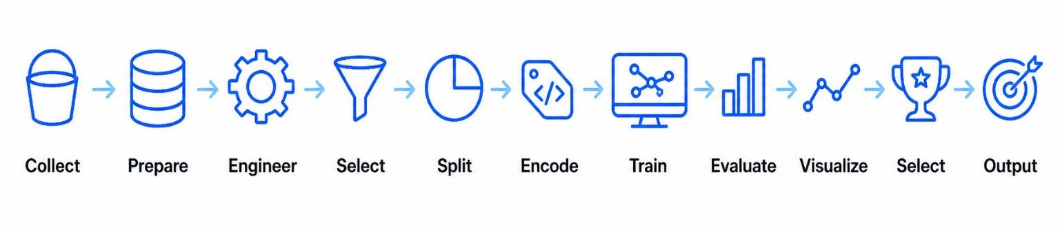
5. End-to-End Workflow
5.1 Data Collection
The dataset is obtained from Kaggle and comprises order-level delivery information, including pricing, item count, store characteristics, and estimated delivery durations. This dataset serves as the foundation for supervised learning.
5.2 Data Preprocessing
Data preprocessing is performed to ensure consistency and correctness of the dataset. Data types are standardized by converting variables into appropriate formats, including numerical, categorical, and datetime types. This step ensures compatibility with subsequent feature engineering and modeling processes.
5.3 Feature Engineering
Feature engineering is applied to enhance model expressiveness and predictive capability. The target variable, delivery time (minutes), is derived from available features created to represent the total duration of each order. Additionally, temporal features such as order hour are extracted to capture demand patterns. Further transformations are performed to encode behavioral trends influencing delivery time.
5.4 Feature Selection
A subset of relevant features is selected to reduce dimensionality and improve model efficiency. The final set of predictors includes subtotal, total number of items, maximum item price, total outstanding orders, estimated driving duration, store category, and order protocol, as these variables significantly influence delivery time prediction.
5.5 Model Development (Split, Encode, Train)
The dataset is partitioned into training and testing subsets using an 80:20 split to ensure unbiased evaluation on unseen data. Categorical variables are then transformed into numerical representations using encoding techniques such as One-Hot Encoding with machine learning algorithms. Subsequently, multiple regression models, including Linear Regression, Random Forest, and XGBoost, are trained to identify the most effective approach for delivery time prediction.
5.6 Model Evaluation and Visualization
Model performance is assessed using standard regression metrics, including Mean Absolute Error (MAE), Root Mean Squared Error (RMSE), and the Coefficient of Determination (R²), providing a comprehensive evaluation of prediction accuracy and variance. In addition, analytical visualizations such as actual versus predicted value plots, feature importance analysis, and residual error distribution are utilized to interpret model performance, supporting both validation and explainability.
5.7 Model Finalization
Based on evaluation results, XGBoost is selected as the final model due to its superior predictive performance and ability to model complex nonlinear relationships.
6. Dataset Description
6.1 Dataset Summary
The dataset is sourced from Kaggle and represents delivery operations from Porter, an intra-city logistics platform. Each record corresponds to a single delivery instance and captures key aspects such as order details, store characteristics, and operational conditions. The dataset is structured and suitable for regression analysis, where the objective is to predict delivery time based on multiple influencing factors.
6.2 Dataset Overview
The dataset consists of operational and transactional data related to food delivery orders.
Total Records: 175,777
Total Features: 14
6.3 Categorical Features
market_id: Identifier for the market or city in which the order was placed
store_id: Unique identifier for the store or restaurant
store_primary_category: Category of the store, typically representing cuisine type
order_protocol: Identifier indicating the method used to place the order
6.4 Numerical Features
total_items: Total number of items included in the order
subtotal: Total monetary value of the order
num_distinct_items: Number of unique items in the order
min_item_price: Minimum price among items in the order
max_item_price: Maximum price among items in the order
total_onshift_dashers: Number of delivery partners available at the time of the order
total_busy_dashers: Number of delivery partners currently occupied
total_outstanding_orders: Number of active or pending orders at that time
estimated_store_to_consumer_driving_duration: Estimated driving time between the store and the customer (in seconds)
6.5 Temporal Features
`created_at: Timestamp indicating when the order was created
actual_delivery_time: Timestamp representing when the order was delivered
6.6 Target Variable
The target variable in this study is delivery time, defined as the total duration between order creation and actual delivery. It represents the time taken to complete a delivery and serves as the dependent variable for the prediction task.
Mathematically, the target variable can be expressed as:
Delivery Time = Actual Delivery Time − Created at
7. Feature Engineering
Feature engineering is applied to transform raw data into meaningful inputs for the model. Since the dataset does not directly provide delivery duration, the target variable is created by calculating the difference between the order creation time and the actual delivery time.
Temporal features are extracted from the created_at timestamp, such as the hour of the day and day of the week, to capture time-based patterns in delivery performance. Categorical variables like store_primary_category and order_protocol are converted into appropriate formats for model compatibility.
8. Exploratory Data Analysis
8.1 Target Variable Analysis
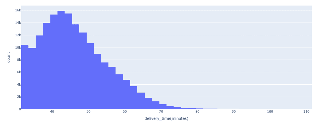
The dataset contains 175,777 records, with an average delivery time of 46.2 minutes and a median of 45 minutes, indicating a fairly consistent delivery duration. Most deliveries fall within the 39 to 52 minutes range, with a standard deviation of 9.33 minutes.
The distribution is slightly right-skewed, showing that while most deliveries are completed within a reasonable time, a small number experience longer delays (up to 110 minutes).
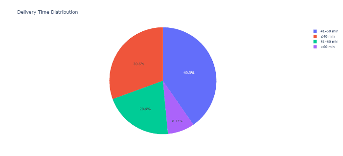
30.6% deliveries ≤ 40 minutes
40.4% between 41–50 minutes
20.9% between 51–60 minutes
8.1% > 60 minutes
Overall, the majority of deliveries are completed within 40–50 minutes, with relatively few extreme delays, making this target variable suitable for predictive modeling and performance optimization.
8.2 Univariate Numerical Features Analysis
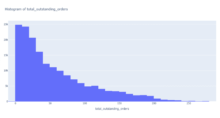
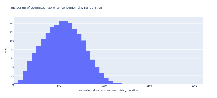
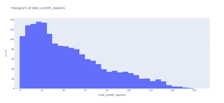
8.2.1 Total Outstanding Orders
The distribution of total outstanding orders is highly right-skewed, indicating that most observations correspond to relatively low order volumes, while a small number of instances exhibit extremely high demand.
This suggests that order congestion is typically moderate but occasionally spikes, likely during peak hours or high-demand periods. Such skewness highlights the importance of handling peak-load scenarios, as these outliers can significantly impact delivery time predictions.
8.2.2 Total Onshift Dashers
The distribution of on-shift dashers also shows a right-skewed pattern, though less extreme compared to outstanding orders. Most values are concentrated in the lower-to-mid range, with fewer instances of very high dasher availability.
This indicates that while supply (dashers) generally remains stable, it may not always scale proportionally with sudden increases in demand. This imbalance between demand and supply can contribute to delays, making this feature highly relevant for predictive modeling.
8.2.3 Estimated Store-to-Consumer Driving Duration
In contrast, the driving duration feature exhibits a near-normal (bell-shaped) distribution, centered around a moderate range of values. This suggests that delivery distances and travel times are relatively consistent across most orders, with fewer extreme cases.
The symmetric nature of this distribution indicates that this feature is well-behaved and less prone to extreme outliers, making it a reliable predictor in the model.
8.2.4 Overall Insights
The presence of right-skewness in demand and supply features indicates variability and occasional extreme conditions, which are crucial for capturing real-world delivery dynamics.
The contrast between skewed (orders, dashers) and normally distributed (driving duration) features highlights different underlying patterns—operational variability vs. geographical consistency.
These distributions suggest that feature scaling or transformation (e.g., log transformation) may be beneficial for skewed variables to improve model performance (especially for Linear Regression).
8.3 Correlation Heatmap of Numerical Columns
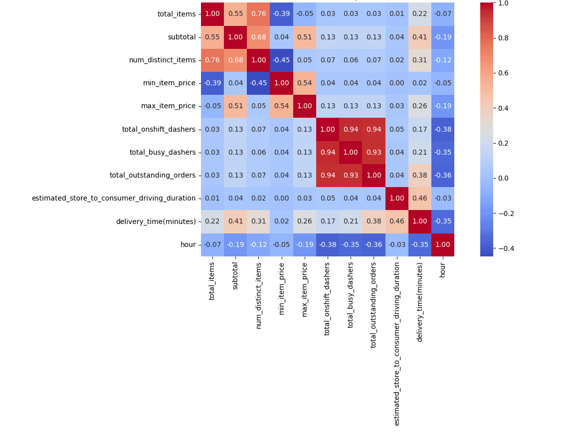
A correlation heatmap was used to examine relationships among numerical variables and their association with the target variable, delivery_time (minutes). This helps identify key drivers of delivery performance and detect multicollinearity.
Estimated driving duration shows the strongest positive correlation (≈ 0.46), making it the most important factor influencing delivery time. Total outstanding orders (≈ 0.38), subtotal (≈ 0.41), and number of distinct items (≈ 0.31) also have moderate positive correlations, indicating that higher demand and more complex orders increase delivery time.
The hour of the day has a negative correlation (≈ -0.35), suggesting improved efficiency during later hours. Dasher-related features show weak positive correlations due to simultaneous increases in both demand and supply during peak periods.
Multicollinearity
Strong correlations are observed among dasher-related and order-related features, indicating overlapping information and shared representation of system load. While this may affect linear models, tree-based models like Random Forest and XGBoost can handle such relationships effectively.
Overall, delivery time is mainly influenced by travel duration, order volume, and order complexity, with temporal factors also playing a role. These insights guided feature selection and model choice.
8.4 Scatter Plot: Operational Factors vs Delivery Time
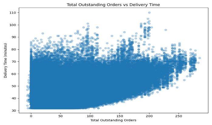
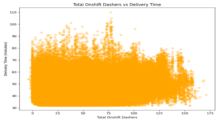
The first plot, Total Outstanding Orders vs Delivery Time, indicates a positive association between order volume and delivery time. As the number of outstanding orders increases, delivery time tends to rise, reflecting congestion effects during high-demand periods. This suggests that system load plays a critical role in delivery efficiency.
The second plot, Total Onshift Dashers vs Delivery Time, shows a negative relationship between the number of active dashers and delivery time. Higher availability of delivery personnel is associated with reduced delivery duration, highlighting the importance of supply-side optimization.
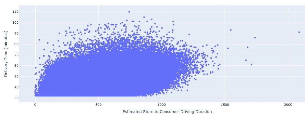
The third plot, Estimated Store-to-Consumer Driving Duration vs Delivery Time, demonstrates the strongest and most direct relationship. Delivery time increases consistently with driving duration, confirming this feature as a primary determinant of overall delivery performance.
8.5 Categorical vs Target Variable
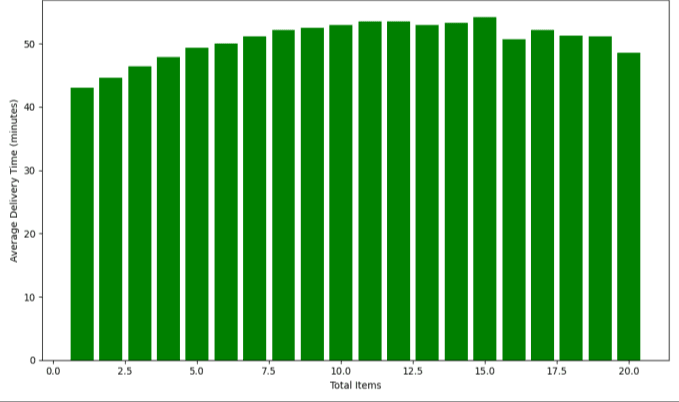
The analysis of Total Items vs Delivery Time reveals a moderate positive trend, where delivery time increases as the number of items in an order rises. This behavior is expected, as larger orders typically require more preparation time at the store, leading to longer overall delivery durations. However, the increase is gradual, suggesting that while order size contributes to delays, its impact is less dominant compared to distance or system load.
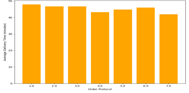
In contrast, the Order Protocol vs Delivery Time plot shows relatively minor variation in average delivery time across different protocol categories. While certain protocols exhibit slightly lower or higher delivery durations, the differences are not substantial, indicating that order protocol has a limited influence on delivery efficiency in comparison to other operational factors.
9. End-to-End Machine Learning Approach for Delivery Time Prediction
9.1 Linear Regression Approach
9.1.1 Feature Selection
Feature variable (X):
subtotal
total_items
max_item_price
total_outstanding_orders
estimated_store_to_consumer_driving_duration
hours
store_primary_category
Target Variable (y):
- delivery_time (minutes)
9.1.2 Train-Test Split and Feature Transformation
To evaluate model performance on unseen data, the dataset was partitioned into training and testing subsets. A larger portion of the data was allocated for training to enable the model to effectively learn underlying patterns, while a sufficiently large holdout set was retained for unbiased evaluation.
Log transformation
Logarithmic transformation was applied to skewed numerical features to stabilize variance and reduce the impact of extreme values:
subtotal
total_items
max_item_price
total_outstanding_orders
Categorical Feature
The categorical feature was transformed into multiple binary (dummy) variables using one-hot encoding. This allows the model to incorporate categorical information without introducing ordinal relationships.
- store_primary_category
9.2 Random Forest and XGBoost Approach
9.2.1 Feature Selection
Feature variable (X):
subtotal
total_items
num_distinct_items
max_item_price
total_onshift_dashers
total_busy_dashers
total_outstanding_orders
hours
store_primary_category
order_protocol
Target Variable (y):
- delivery_time (minutes)
9.2.2 Train-Test Split and Feature Transformation
To evaluate model performance on unseen data, the dataset was partitioned into training and testing subsets. A larger portion of the data was allocated for training to enable the model to effectively learn underlying patterns, while a sufficiently large holdout set was retained for unbiased evaluation.
Categorical Feature
The categorical feature was transformed into multiple binary (dummy) variables using one-hot encoding. This allows the model to incorporate categorical information without introducing ordinal relationships.
- store_primary_category
10. Model Evaluation
10.1 Baseline Model Evaluation — Linear Regression
The RMSE of approximately 7 minutes indicates the average deviation between predicted and actual delivery times.
The R² score suggests that around 42.5% of the variance in delivery time is explained by the model. While the model captures general trends in the data, a significant portion of variability remains unexplained.
Table: Linear Regression Metrics
| Metric | Value |
|---|---|
| MSE | 50.27 |
| RMSE | 7.09 |
| R2_SCORE | 0.425 |
10.2 Ensemble Model Evaluation — Random Forest
The RMSE of approximately 2.56 minutes indicates that the average deviation between predicted and actual delivery times is significantly low, reflecting high prediction accuracy.
The R² score suggests that around 92.5% of the variance in delivery time is explained by the model, indicating strong explanatory power.
Unlike Linear Regression, the model captures complex patterns in the data, resulting in predictions that closely align with actual values. The low error and high variance explanation demonstrate that the model effectively learns both linear and non-linear relationships, with only a small portion of variability remaining unexplained.
Table: Random Forest Metrics
| Metric | Value |
|---|---|
| MSE | 6.55 |
| RMSE | 2.56 |
| R2_SCORE | 0.9249 |
10.3 Ensemble Model Evaluation — XGBoost
The RMSE of approximately 2.37 minutes indicates that the average deviation between predicted and actual delivery times is very low, reflecting high prediction accuracy.
The R² score suggests that around 93.6% of the variance in delivery time is explained by the model, indicating excellent explanatory power.
Compared to Random Forest, XGBoost demonstrates a slight improvement in both error reduction and variance explanation, highlighting its ability to optimize predictions more effectively.
Table: XGBoost Metrics
| Metric | Value |
|---|---|
| MSE | 5.61 |
| RMSE | 2.37 |
| R2_SCORE | 0.9359 |
The model captures complex non-linear relationships and interactions between features, resulting in predictions that closely align with actual delivery times. Only a minimal portion of variability remains unexplained.
11. Model Performance Analysis
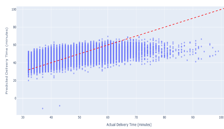
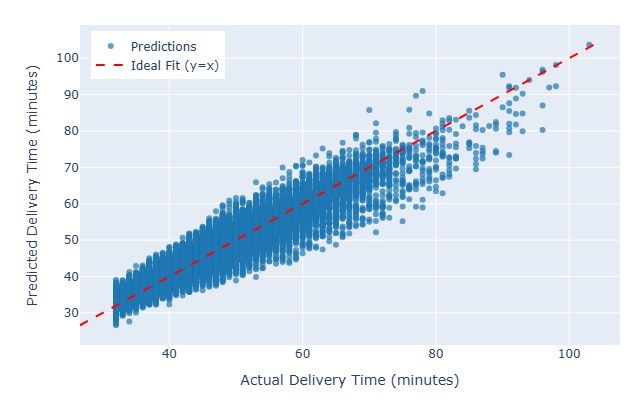
Figure 1.9 presents a comparative evaluation of Linear Regression and XGBoost models using Actual vs Predicted delivery times. The diagonal reference line (y = x) represents the ideal scenario where predicted values perfectly match actual delivery times.
The Linear Regression model (left plot) demonstrates a clear limitation in capturing the variability of delivery times. Predictions are concentrated within a narrow band, indicating that the model tends to underfit the data. As actual delivery times increase, the model fails to proportionally adjust its predictions, resulting in systematic deviations from the ideal line. This suggests that the linear assumption is insufficient for modeling the inherent complexity and non-linearity in delivery time dynamics.
In contrast, the XGBoost model (right plot) exhibits significantly improved alignment with the ideal fit line. The predictions are more widely distributed along the diagonal, indicating that the model effectively captures both linear and non-linear relationships within the data. The reduced dispersion around the reference line highlights better predictive accuracy and robustness across varying delivery time ranges.
Overall, the visual comparison clearly indicates that XGBoost outperforms Linear Regression, providing more reliable and accurate predictions. This improvement can be attributed to XGBoost's ability to model complex interactions and handle non-linear patterns, making it a more suitable choice for real-world delivery time estimation tasks.
12. Model Feature Importance Analysis
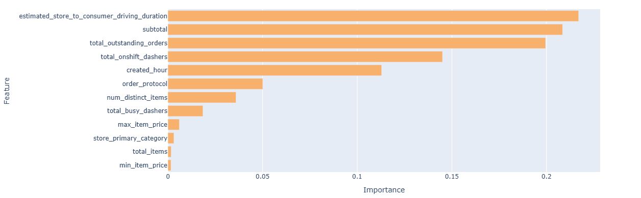
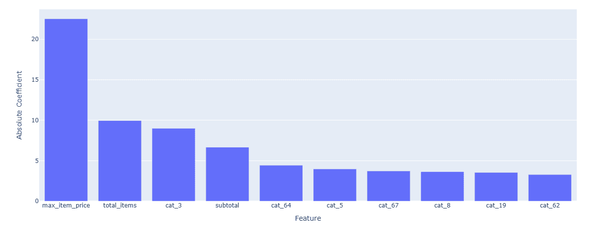
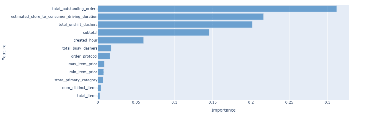
Feature importance analysis reveals that estimated driving duration and total outstanding orders are the most influential predictors across ensemble models. This highlights that both geographical distance and system congestion are primary drivers of delivery time.
13. Conclusion
XGBoost emerges as the final optimized model, achieving the highest accuracy and most reliable predictions. Its ability to model complex delivery dynamics makes it the most suitable approach for this problem.
14. Future Work
Future improvements can include incorporating real-world factors such as traffic, weather, and location data to enhance prediction accuracy. The model can also be extended into a real-time system for dynamic delivery time estimation. Additionally, further feature engineering, model optimization, and explainability techniques can be explored to improve performance and reliability. Deployment at scale using cloud-based systems can enable practical, real-world application.
References
- Porter Delivery Time Estimation Dataset: https://www.kaggle.com/datasets/ranitsarkar01/porter-delivery-time-estimation-dataset/data
- End to End Analysis:
- Hastie, T., Tibshirani, R., & Friedman, J. (2009). The Elements of Statistical Learning. Springer.
- Draper, N. R. & Smith, H. (1998). Applied Regression Analysis. Wiley.
- Kuhn, M. & Johnson, K. (2013). Applied Predictive Modeling. Springer.
- Molnar, C. (2020). Interpretable Machine Learning. Lulu Press.
- Friedman, J. H. (2001). Greedy Function Approximation: A Gradient Boosting Machine. Annals of Statistics.
Terno AI chat share links:
https://port.app.terno.ai/chat/share/1d8d5aed-8a16-41da-a819-6bc4e3237dac?ui_version=v2
https://port.app.terno.ai/chat/share/02a9dbd5-0b80-42ca-a256-9557d095a78a?ui_version=v2
Read the full whitepaper

18 August 2026
The Honest Number Was 83%: Leakage, Abstention, and a Complaint Router You Can Actually Deploy
The same complaint-routing model scores 96.3% or 83.2% depending on which three columns you leave in the training data. The high number is the intake form being read back to you. This is what the leakage audit found before a single model was trained, why 83.2% is the honest figure, and how the same model — given permission to say "I don't know" — becomes deployable at 90.7% accuracy on 79.5% of traffic.

29 July 2026
EdgeGuard: AI-Driven Predictive Maintenance for Power Transformers
Power transformers are among the most critical assets in electrical distribution infrastructure. Their unexpected failure can result in power outages, safety hazards, equipment damage, expensive repairs, and long service interruptions. Traditional transformer maintenance practices often rely on periodic manual inspection, offline testing, or run-to-failure maintenance. These methods are expensive, slow, labor-intensive, and unable to detect rapidly developing faults in real time. EdgeGuard is an AI-driven, edge-computing predictive maintenance system designed to continuously monitor transformer health and forecast failures before catastrophic damage occurs. The system acts as a retrofittable “Digital Doctor” for distribution transformers by combining low-cost industrial sensors, an ESP32 microcontroller, local intelligence, machine learning-based risk prediction, autonomous relay control, and a real-time web dashboard. The proposed system monitors six major transformer health indicators: temperature, humidity, vibration, oil level, current, and voltage. These signals are normalized and processed through a Multi-Layer Perceptron neural network to classify transformer condition and estimate failure risk. If the predicted risk crosses a critical threshold of 80%, EdgeGuard automatically triggers a relay through GPIO 26 to isolate the transformer from the electrical network. The system also supports secure remote control, dashboard monitoring, API-key-based hardware authentication, JWT-based user access, WebSocket live updates, and automatic live-hardware detection. With an estimated deployment cost of approximately ₹3,850, EdgeGuard offers a low-cost alternative to conventional transformer monitoring systems. Its cloud-independent operation and edge-based decision-making make it especially useful for rural and semi-urban distribution grids where connectivity and maintenance resources are limited.

28 July 2026
ANALYZING TOXIC USER BEHAVIOR AND RISK PATTERNS IN ONLINE GAMING PLATFORMS
This study shows that behavioral data alone can't reliably predict gaming toxicity — but a risk-based model combining behavioral and engineered features does a much better job of flagging the small segment of high-risk users driving disproportionate harm.